1:45 pace

2:15 pace

2:00 pace

Crap-shoot modeling

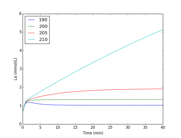
I published a crap-shoot lactate kinetics model on my training blog.

“Pull” vs “Push” Recovery – some thoughts

I was triggered to look again at my recovery profile calculations by the discussion on Ben Redman’s blog, with a reference to this article on the Rowing in Motion website. Basically, the thinking is that by optimizing the recovery profile and trying to accelerate on the slide as long as possible during the recovery (by “pulling on the footstretcher”) one can gain speed, as opposed to decelerating early and approaching the catch slower (“pushing on the footstretcher”). There seems to be some empirical evidence from Kleshnev (RBN 140) that “Olympic champions” have a more pronounced boat deceleration at the catch and a later point in the recovery where the boat acceleration becomes negative.

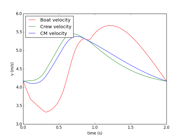
I did some simulations at 30spm using a three different (quite extreme) recovery profiles. In the following plots the red curve is the (measurable) boat velocity, the green curve is the crew velocity and the blue curve is the velocity of the center of mass. The stroke force profile is the same in all three simulations.

Recovery 2: Boat, crew and system speed

Recovery 3: Boat, crew and system speed

Recovery 1: Boat, crew and system speed

In all three cases, we achieved the following results (for a single sculler of 80kg rowing in a 14kg boat with a fairly conservative rigging):

Average speed achieved: 4.70 m/s (in rowing terms a 1:46.3 pace)
Average stroke power: 490W

At constant stroke rate and with a similar average speed, there isn’t much variation possible in the recovery style. One simply has to return the handles form the finish position to the catch position in a given amount of time. At constant stroke length, the average handle speed will be a given. So either you “pull” a bit more in the beginning and then cruise, or you pull less in the beginning of the recovery and keep pulling. You can see that there is not much difference in the blue curves for the center of mass. The speed decrease is caused by the drag force on the hull, which is higher at higher boat speed, but as the average recovery speed is a given, the average boat speed is also a given, and even though we are dealing with a non-linear system, the differences are negligible.

The Rowing in Motion article gives this picture (admittedly, in the comments warning that it is “for illustration purposes only”):

It is very tempting to use hand-waving arguments based on feel in discussions on rowing physics.You have to realize though that a quick illustration as the one above can never be accurate. For example, the graph clearly doesn’t show steady state, as the boat speed is 1 m/s higher at the end of the stroke. I am also wondering, if you would calculate a speed profile for the rower that would produce these two curves, if you would arrive at the same stroke length. Are we comparing apples and pears?

You have to keep thinking about underlying principles, about whether or not something is significant, and about whether or not there is an alternative explanation for something that is “found” empirically. In RBN 140, Kleshnev discusses some very interesting observations, but I think more studies will be necessary to figure out exactly if (and how) this contributes to the boat speed of Olympic rowers. We may even have cause and effect in the wrong order. Those Olympians also tend to be the ones able to row longer at higher power and stroke rates. There may also be differences in stroke length and posture benefiting boat speed which cause the features described in the Kleshnev paper.

Stroke Profile Continued

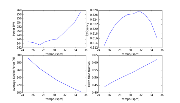
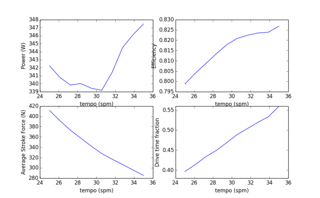
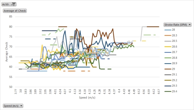
I have been trying to find some artificial stroke profiles that come close to simulate my measured acceleration on a 30 spm stroke (measured with Rowing in Motion). Then I did 4 quite coarse variations to that stroke profile and ran a simulation for 25 to 35 spm using those profiles. Here are the stroke profiles I used:

The stroke profiles used in the simulation

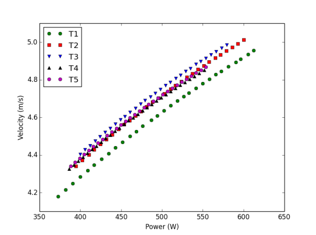
Simulating the power-velocity graphs for these strokes gives the following result:

Average Boat Speed vs Average Power Consumption

So T3 is better than T2, T4 and T5 which are roughly equal, and all are better than T1. Again, we have to remember that these values depend on the catch angle and I need to rerun the simulation for a different catch angle, which I took at 63 degrees for this simulation.

Here is what CrewNerd check would give:

Crewnerd Check numbers

The actual check values in CrewNerd would be different, but I am using the equivalent formula, just scaled, that CrewNerd is using. Lower check is better, so we have roughly two situations:

At lower stroke rates, T3, T4 and T5 are “best”, T2 is in the middle and “T1” is the worst
At higher stroke rates T3 is the best, followed by T2, T4, T5 and T1

In conclusion, for this setting, CrewNerd Check factor would give the right feedback. If you would be able to reduce check at constant speed, you are probably moving to a more economic stroke profile.

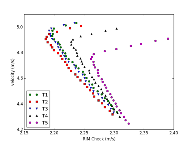
The RIM Check metric has a similar name but is calculated differently:

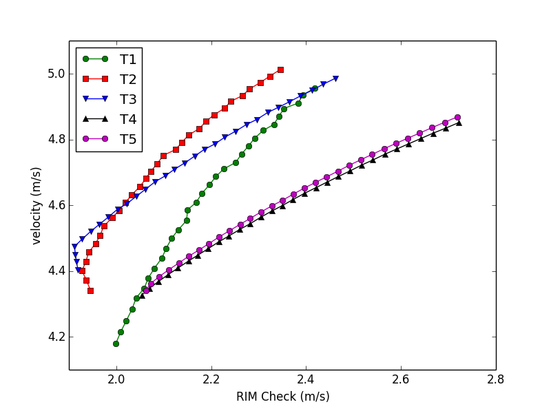
RIM check vs average boat speed

So here, roughly, T2 is the best, followed by T3, then T1 and finally T4 and T5. Something weird is going on with T1. Looking at the stroke velocity plot at 30spm, it is clear:

Speed vs time for one stroke with T1 profile

I guess the simulation is not entirely realistic here around the catch (between 0 and 0.15 seconds in the graph). Such a profile is not realistic in a real boat.

Finally, I will look at RIM “stroke efficiency”:

RIM Stroke Efficiency vs Speed

Here, a higher value is better. So we have T1>T5>T4=T2>T3. This looks like the exact opposite of what we should get. This parameter depends a lot on the value of the minimum velocity. For the stroke profiles I have chosen that minimum velocity is determined really by the force around and immediately after the catch. By “checking” the boat (meaning pushing hard on the footstretcher around the catch) we are making this a low value, which helps the parameter, which is a double integral of boat acceleration, so quite sensitive to calibration accuracies in the RIM app.

So it seems it will be better to look at RIM Check or CrewNerd check for live technique feedback in the boat.

Next, I am going to rerun the simulations looking at catch angle.

Data Spaghetti (Thursday session)

A rowing physics (data) related blog on my regular training blog.

Updated the model

Triggered by the interesting discussions (https://forum.rowinginmotion.com/) and the availability of measured data, I have recently spent some time on updating my model.

It was never my intention to make a super detailed model that would be able to reproduce each and every speed and acceleration peak and valley from a measurement on a real rower. Instead, I wanted to make it just realistic enough to be able to play with the parameters and see how they effect rowing efficiency, in order to trigger some discussions about rowing technique and rowing style.

Here is the algorithm flow of my original model (see https://sanderroosendaal.wordpress.com/2010/07/13/calculating-a-single-stroke/):

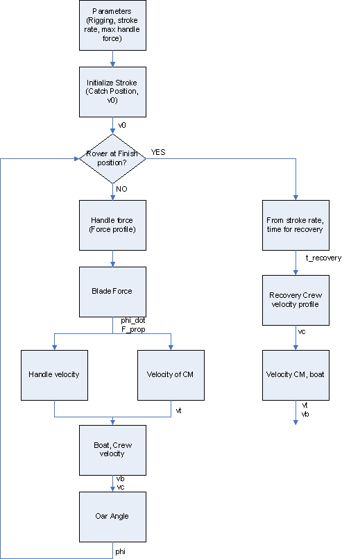
The original algorithm to calculate one stroke

The flaw was that the boat speed made a jump from finish to catch because in my model,

the rower center of mass velocity at the finish was zero
the rower center of mass velocity at the catch was dictated by the handle speed to generate the correct handle force

What happens in reality of course is that one places the blade a fraction of a second after one reverses the body CM velocity. There were two ways to improve this. First, I added some “generic” recovery profiles which would be able to simulate that fraction of a second as part of the recovery phase of the stroke.

Nothing wrong with that approach, except that it was difficult to calculate a recovery profile which generated the right “catch CM speed”, with the right stroke length and everything. I still have provisions for this in my software, so once I have some time I can start using this route.

For now, I have patched the algorithm on the “stroke” side. I added a “catch” phase at the beginning of it. Here is the revised algorithm:

What I do is the following. During the catch phase I make 2 calculations:

Accelerate rower Center of Mass without placing the blade, and calculate subsequent boat, crew velocities, oar angle, and some other parameters
Calculate what the rower Center of Mass would be if he/she placed the blade at this moment in time

The blade is “placed” at the moment that these two velocities are equal (or, to be precise, at the moment that the velocity before placing the blade starts to exceed the velocity if the blade had been placed).

In rowing terms this moment of placing the blade would generate a beautiful V-shaped splash. Too early, you have a front splash and are stopping the boat. Too late and you are missing water and have a back splash.

The picture shows a typical stroke. So now I have continuous velocity profiles. I still have jumps in acceleration, where in a real system also the acceleration change would be smooth, but for the moment I consider it not necessary to make my model that realistic.

Of course I was interested to know if this improvement would invalidate any of my previous published results, so I reran all simulations of previous blog posts (and some more). I am happy to report that everything still holds.

Stroke Metrics

For OTW stroke metrics, there are two interesting applications, RIM (http://www.rowinginmotion.com/) and Crewnerd (http://performancephones.com/crewnerd/).

Crewnerd gives a “check factor” metric of how well you are rowing. RIM has several metrics. Today I will discuss “stroke efficiency” and “check factor”.

I was interested to see what my model had to say about these metrics. Be aware that this post may tell as much about the imperfections of my model as about those two apps.

In this post I am going to look at the metrics for different force profiles during the stroke. These are the stroke force profiles I am using:

The ultimate efficiency measure of rowing is to get the maximum average boat speed at a given power. The below picture is a key picture calculates just that. The differences between the different stroke profiles are quite subtle.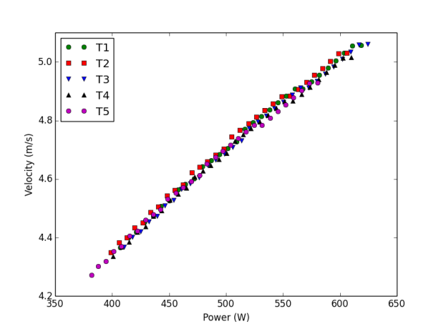

So what does the graph tell us? First, that the differences in speed are very subtle. Still, it seems that red circles (T2) are the most efficient, lowest average power at a given average boat speed. Profile T5 seems to be the worst.

So how does Crewnerd’s “Check Factor” look like?

T5 is clearly the worst, giving the highest value of “check” at a given boat speed.

What is also clear is that to increase speed, one ends up inevitably with a higher value of “check”. Don’t try to minimize check at the cost of losing speed!

Now we turn to RIM. The RIM definition of “check” is just the difference between max and min boat speed.

So, at a given velocity, T2 is clearly the “lowest check” value and T5 the worst. It seems also RIM definition of “check” is useful.

RIM has another metric, “stroke efficiency”, defined as the integral of boat speed over one stroke, minus the integral of minimum boat speed. It measures how much further your stroke takes you compared to the minimum boat speed.

For this metric, higher is better. So again T5 scores the worst, and the best seems to be T3.

I think it is too early for conclusions, but here are some take away messages that I stick to for now:

Expect any metric to change with boat speed and stroke rate. You should make sure you keep both constant if you try to optimize your stroke, which is difficult
At given boat speed and stroke rate, the three tested metrics are consistent in the sense that optimizing them brings you to the most efficient power profile.

To be continued …

New Rowing Physics and Rowing Mechanics Forum

This blog with my attempts to model Rowing Physics has been collecting dust for a while. I intend to keep these pages for reference and will publish new blog posts whenever I develop new functions or improve it.

However, I would really love to move the discussion on Rowing Physics and the comparison of the different models out there to this new Forum: https://forum.rowinginmotion.com/

Why?

We are starting to see the possibilities for low-cost easy-to-access empirical data driven approaches. This is very exciting. The above-mentioned blog is maintained by the developer of Rowing in Motion who is very active. Let’s all move to where the action is!!!

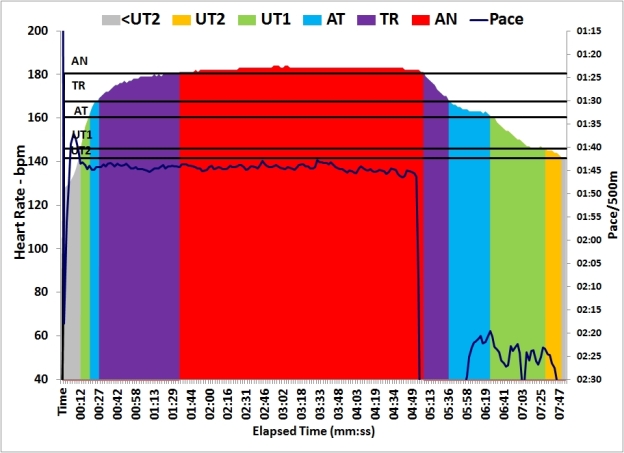
Carole McNally Memorial CTC and 2k tester

Workout Summary – Feb 14, 2015

–|Total|-Total-|–Avg–|-Avg-|Avg-|-Avg-|-Max-|-Avg|-Avg

–|Dist-|-Time–|-Pace–|Watts|SPM-|-HR–|-HR–|-DPS|-SPI

–|02000|07:58.1|01:59.5|205.0|27.4|172.5|184.0|09.2|07.5

Workout Details

01|00100|00:20.8|01:43.8|312.8|31.8|140.3|159.0|09.1|09.8|

02|00100|00:20.8|01:44.1|310.1|31.7|169.3|174.0|09.1|09.8|

03|00100|00:20.8|01:44.2|309.2|31.7|176.6|178.0|09.1|09.8|

04|00100|00:20.9|01:44.7|305.0|31.5|179.3|180.0|09.1|09.7|

05|00100|00:20.8|01:44.0|310.9|28.8|180.4|181.0|10.0|10.8|

06|00100|00:20.9|01:44.6|305.6|31.5|181.6|182.0|09.1|09.7|

07|00100|00:20.9|01:44.3|308.4|31.6|182.0|182.0|09.1|09.7|

08|00100|00:20.8|01:44.2|309.7|31.7|183.0|183.0|09.1|09.8|

09|00100|00:20.9|01:44.3|308.6|28.8|183.4|184.0|10.0|10.7|

10|00100|00:20.9|01:44.4|308.0|31.6|183.1|184.0|09.1|09.7|

11|00100|00:20.7|01:43.7|314.2|31.8|183.0|183.0|09.1|09.9|

12|00100|00:21.0|01:45.0|302.4|31.4|183.0|183.0|09.1|09.6|

13|00100|00:21.0|01:45.2|300.7|31.4|183.0|183.0|09.1|09.6|

14|00102|00:21.5|01:45.6|297.5|33.4|182.6|183.0|08.5|08.9|

15|00098|00:37.8|03:13.1|048.6|17.4|177.8|182.0|08.9|02.8|

16|00500|02:27.4|02:27.4|109.3|22.0|155.5|171.0|09.3|05.0|

Fletcher Warming up, followed by a 2k, of which I rowed only the first 1402m at my estimated 2k pace. Predicted end time just under 7 minutes.

A model of rowing

Numerical Modeling of the physics of rowing